PhD Research
Below are the projects from my doctoral dissertation, which focuses on computational mathematics and fluid dynamics. The main focus of the dissertation is a fast mesh-free boundary integral method for two-phase flow with soluble surfactant. The secondary focus of the dissertation is a study of electroconvective flow. For a closer look at the movies, please see the videos page.
A fast mesh-free boundary integral method for two phase flow with soluble surfactant
The primary focus of my dissertation was on the development of a fast mesh-free boundary integral method for two phase flow with soluble surfactant. Surfactant is a surface-active agent that lowers the surface tension and introduces forces that affect interfacial evolution and can lead to rich dynamics. Surfactants are very common as they are often used in foaming agents and emulsifying agents, and are also important in microfluidic applications which refers to the study of fluid systems with small length scales.
Numerical studies of interfacial flow with surfactant commonly simplify the dynamics by assuming the surfactant is insoluble, i.e., restricted to the surface alone. In this case, spectrally accurate boundary integral methods can be employed to simulate the interface evolution (Pozrikidis 1992 and Palson, Siegel and Tornberg 2019). These are among the most accurate and efficient methods for solving Stokes flow problems. However, it is difficult to adapt boundary integral methods to problems with soluble surfactant as the advection-diffusion equation for the bulk surfactant does not have a Green’s function formulation. In addition, at large Peclet numbers Pe that are characteristic of real physical systems, the concentration of soluble surfactant develops a transition or boundary layer adjacent to the drop surface which is difficult to resolve using traditional numerical methods. Previous numerical studies of multi phase flow with soluble surfactant have employed front tracking (Muradoglu and Tryggvason 2008) and embedded boundary methods (Khatri and Tornberg 2014). However, these methods are only low order accurate and need to employ artificially small Pe to resolve the boundary layer.
To address the difficulties, in my thesis a ’hybrid’ numerical method that was first introduced in Booty and Siegel (2010) and extended to two-phase flow with soluble surfactant in Xu, Booty, and Siegel (2013) is further developed. The hybrid method is based on an asymptotic reduction of the surfactant dynamics in the transition layer in the limit Pe → ∞. This reduced advection-diffusion equation for the concentration of bulk soluble surfactant has a Green’s function formulation. A fast method for computing a time-convolution integral that arises in the Green’s function formulation of the advection-diffusion equation is introduced. There are several challenges in developing the fast method, which is based on a method originally introduced for Abel integral equations by Johannes Tausch (2010).
Consider the canonical example of a single viscous drop of fluid immersed in a viscous surrounding fluid and deformed by an imposed external flow. Both fluids are immiscible Newtonian fluids, and we focus on the low Reynolds number limit leading to incompressible Stokes flow as well as the large Peclet number limit. The figure below depicts the bulk concentration of surfactant of a deformed drop, as well as a close up of one of the drop tips. The flow causes the surface surfactant to accumulate at the tips, which then desorbs from the surface due to solubility. Conversely, surfactant is pulled across the transition layer and absorbs onto the drop surface in regions where the drop shape is relatively flat and the concentrations are lower.
In comparison to traditional algorithms that discretize the fluid region using a boundary fitted mesh, the spectral method developed in my thesis is better able to handle thin boundary layers at large Pe, as well as unbounded external flow domains. The hybrid method uses the Sherman-Lauricella boundary integral formulation to give fluid velocity in terms of the surface concentration of surfactant and interface shape. The method is considered mesh free as no spatial mesh in the normal direction is needed to solve the transition layer. The concentration of soluble surfactant in the transition layer is instead represented by a Green’s function formulation which takes the form of a time-convolution integral similar to that for the heat equation but with a more complicated kernel.
The main challenge is to develop a fast method for computation of this Abel-type convolution of the form
A significant complication is that both the kernel k(t,τ) and the density g(τ) are not known in advance, but depend on the solution of a system of time-evolution equations. In collaboration with Johannes Tausch (SMU), we have developed a fast algorithm that overcomes these difficulties by adapting a fast method for the evaluation of Abel-type convolution integrals first developed in Tausch (2010). While fast algorithms of this type have previously been developed for the heat equation (Tausch 2007), we believe this is the first instance of such an approach for an advection-diffusion equation. We note that the method should be useful in other contexts.
The method was validated against a mesh-based method from Xu, Booty and Siegel (2013) and outperforms that method in terms of speed. It’s overall operation count is O(P log_2 P(m+m^2)) where P is the number of time steps and m is the number of interface grid points. The m^2 comes from the fluid solver for the Sherman-Lauricella equation, and can be made to be O(m) using a fast algorithm such as the fast multipole method (FMM). The method is spectrally accurate in space and has temporal order of accuracy O(h^(3/2)) where h is the time step size. The time accuracy can in principal be improved, which we propose to do in future work. This method provides a novel fast algorithm for advection diffusion.


Validation


The above figrues show the bulk surfactant exchange term at the interface grid points at various times, with a close up correspinding to a drop tip on the right, calculated using our fast mesh-free method (red dots) and the mesh based method (blue curves). The calculation of the bulk surfactant exchange term is the main difference between the two methods, and we can see good agreement between the two methods at all times.
Speed

The table shows the wall clock time for the calculation of the bulk surfactant exchange term using the fast mesh-free method, the mesh-free method without the fast computation of the time convolution integral, and the mesh-based method with various mesh sizes. Going across the rows, we can see that the wall clock time when using the fast mesh free method slightly more than doubles when doubling the number of time steps, hence it is O(PlogP) per interface point where P is the number of time steps. When not using the fast method for the convolution however, the time for the mesh-free method is multiplied by four when the time steps are doubled, meaning it is O(P^2) per interface point. The time for the mesh-based method for all mesh sizes doubles when doubling the number of time steps. However, going down the columns for the various mesh sizes, we can see that as the size of the mesh doubles eventually the time to compute the bulk surfactant exchange term is multiplied by four. This means the overall operation count for the mesh-based method is O(PM^2), where M is the size of the mesh, per interface point. For accuracy, a typical mesh size is M=512. Comparing the fast mesh-free row to the M=512 mesh row we see how well the fast mesh-free outperforms the mesh-based.
Numerical Examples
We also tested our method on different domains, an example of some can be seen here with the C-domain on the right and the swiss-roll domain below. The C-domain is deformed in a shear flow, and over time we can see that it is pulled open into an elliptical shape. We can also see that the flow causes the surface surfactant concentration to congregate to the tips of the drop. However there is high surface concentration of surfactant where the initial tips of the 'C' have evolved to as well. This is because those portions of the drop change the most over the evolution as the interface length decrease, and so the concentration of surfactant is greater.


For the swiss-roll domain we have turned off the imposed far-field flow. This means the forces acting on the drop are the surface tension and the pressure and viscous stress forces. These forces, without the far field flow, cause the drop to relax over time until it ultimately becomes a circle. The left movie shows the surface surfactant concentration as the drop evolves while the right shows the bulk concentration of surfactant. We can see in both, that like in the C-domain, the highest concentrations of surfactant, both bulk and surface, occur where the drop shape has changed the most. In the swiss-roll case this corresponds to the initial tips of the spiral. Once the shape appears circular, the surfactant concentrations will continue to evolve until it is uniform. This is because until the surfactant concentration is uniform there will be slight surface tension remaining even though the drop is ciruclar, which causes the evolution to continue until the surfactant concentration is uniform.
To see the movies more clearly, please see the videos page.
A study of electroconvective flow
Voltage driven transport of ions is present in many electrochemical systems. It is significant in applications such as desalination of water and Lithium-ion batteries. An important and unresolved challenge for turbulent electroconvection is developing reduced order models (Mani and Wang 2020). This is because realistic parameter values require resolving small scales which is currently unfeasible with direct numerical simulations.
Following the approach of Druzgalski, Andersen and Mani (2013), the problem we are considering is that of a symmetric binary electrolyte bounded by an ion selective surface on the bottom and a stationary reservoir on top. The system is periodic in the horizontal direction and wall-bounded in the vertical direction. The ion selective surface is impermeable to anions and a voltage is applied to the stationary reservoir. This difference in electrostatic potential drives the flow. The greater the potential difference the more turbulent the flow becomes. This is due to the ion selective surface rejecting the anions, which brings rise to electroconvection. Electroconvection is a hydrodynamic instability and appears as vortices in the flow.
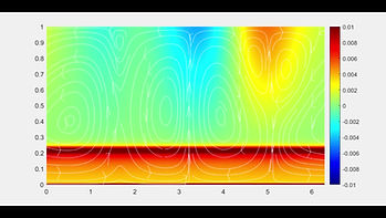
As the applied voltage increases the vortices become less organized and will then eject both positive and negative charge densities into the bulk of the fluid, which is known as electroconvective turbulence. An example of this can be seen in the figure above, which shows a snapshot from our simulation of the model with a high applied voltage of ∆ϕ = 120. The colors represent the charge densities, and the flow streamlines are superimposed. The model is based on the electrostatically forced incompressible Stokes equations coupled to the Poisson-Nernst-Planck equations. The stream function form of the Stokes equations is used, which gives rise to the 2D forced biharmonic equation.
In the closely related Rayleigh-Benard convection, it is a common approach to use a Chebyshev-Fourier representation. However, the round-off error when using the kth Chebyshev differentiation matrix grows like O(N^(2k)δ) where N is the number of discretization points in the vertical direction and δ is machine precision (Don and Solomonoff 1997). This leads to difficulties when a large number of Chebyshev points are used to resolve the flow.
Currently, I am working on comparing a ultraspherical-Fourier representation (Olver and Townsend 2013) to the standard Chebyshev-Fourier representation with Kosloff Tal-Ezer mapping (Kosloff and Tal-Ezer1993). In my dissertation we compared the methods on a synthetic problem, and found the ultraspherical coordinates obtained a much higher accuracy when a large number of discretization points (> 200) is used in the non-periodic direction. We will compare the Chebyshev Fourier Kosloff Tal-Ezer and ultraspherical representations on the full problem. So far we have found that the Kosloff Tal-Ezer mapping is not as accurate as the ultraspherical, as expected. This results in the Kosloff Tal-Ezer representation requiring a smaller time step for stability. Using too many points in the vartical direction with the Kosloff Tal-Ezer mapping is also problematic, as this leads to the derivative matrix in the biharmonic operator for the stream function equation being close to singular.

Our main work, in collaboration with Ioannis Koutis (NJIT CS), is training convolutional neural networks (CNNs) to predict unclosed terms in an approximate (reduced) model of electroconvection. We are interested in the relationship between the applied voltage and the space and time averaged current. Results from our simulations can be seen as the blue circles in the figure to the right. The red curve is the time averaged current without fluid flow. We see a linear relationship in the circle data between ⟨I⟩ and ∆ϕ at sufficiently large voltages. We want to take this further, with greater applied voltages as well as smaller screening length ϵ which is more indicative of practical physical

problems. However the small scales make direct numerical simulation unfeasible due to high computational cost. This is where the CNN enhanced calculation of unclosed terms will come into play. We expect it will allow us to calculate the space and time averaged current without detailed solution to the full system of equations at fine resolution. We are also considering other avenues of machine learning, such as Transformers, to improve computational costs.
Electroconvective Turbulence
Below are two examples of electroconvective turbulence. The left movie shows electroconvective turbulence for an applied voltage of ∆ϕ=40 and the right movie uses ∆ϕ=120. The flow streamlines are superimposed over the charge densities. The difference in electrostatic potential between the top and the bottom drives the flow, and becuase the bottom boundary is ion-selective and does not allow anions to pass through we see electroconvective turbulence arise and positive and negative charge densitites being ejected into the bulk of the fluid. For the higher applied voltage of ∆ϕ=120, we see that the densitites ejected are greater as well as ejected greater distances, and that the flow streamlines are less organized. It is because of this turbulence that more resolution is required in space and time, which is what makes direct numerical simulation of higher voltages with realistic screening length currently unfeasible.

To see the movies more clearly, please see the videos page.